Anatomy of the IMS RINs pricing model
Anatomy, [ə’nadəme] noun – a study of the structure or internal workings of something
The Irwin McCormack Stock (IMS) RINs pricing model is based on fundamental economic and asset pricing theory and has been proven to accurately model real-world D4 RIN prices. In 2020, Hoekstra Trading implemented it in a spreadsheet for use in analyzing, studying, and predicting RIN prices. The equation is:
PD4 = e^(-r√(T-t)) (f0-(f0-f1)(pb+(1-q)(1-b)))/1.5
Here I break down this formula to better understand how it works in pricing a RIN.
Consider a D4 RIN with 1 year life (T-t=1) at a time when the blender’s tax credit is in effect (b=1). Substitute these into the price equation, then for this special case:
PD4= e^(-r)(f0-(f0-f1)p)/1.5
p is the probability the blender’s tax credit will stay in effect. r is the risk-free interest rate. f0 and f1 are functions of the stochastic variable s which depends on the current and future prices of diesel and biodiesel:
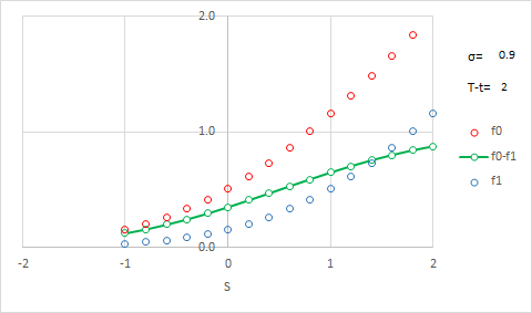
VARIATION OF f0 AND f1 with s
f0 is defined as f0 = σ√(T-t) φ(s/(σ√(T-t)))+sΦ(s/(σ√(T-t)))
σ is the standard deviation of s. Set it =0.9. For a RIN with 1 year until expiration, f0 is the sum of its 1st and 2nd terms:
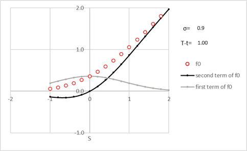
The first term of f0 (gray curve) is a normal density distribution. The second term (black curve) is s multiplied by a cumulative normal distribution. The sum, f0, (red) resembles an option price curve. It approaches asymptotes f0=s along the positive s axis (like a far in the money option) and f0 = 0 as s goes increasingly negative (like a far out of the money option).
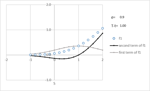
f1 is also defined in the model, it is the same function as f0 but shifted right by $1:
With this breakdown of the formula, the price of a RIN, PD4 , is seen to be a combination of 2 option price curves, one curve for each of 2 states.
The “tugging” effect of uncertainty about the future state:
When b is 1, we can think of the blue curve f1 as the “operative curve” for that current state, and it is being tugged toward the red curve f0 by an amount that is (f0 – f1 )p.[1] The blue curve f1 is capturing the uncertainty about the future value of s, and the “tug term”, (f0 – f1 )p is capturing the uncertainty about the future state of the blender’s tax credit.
The “tug factor”, (f0 – f1), for this special case is the green curve below:
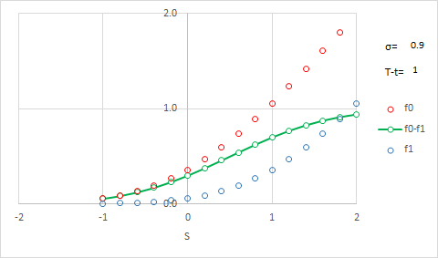
The tug factor resembles the price curve for a $1 vertical option price spread. It approaches 1 as (f0 – f1) increases and it approaches 0 as s goes increasingly negative.
Understanding the equation as consisting of these 3 framework components, two option price curves plus a “tug term”, helps understand how all the model’s variables and parameters affect the RIN price.
Understanding the equation as consisting of these 3 framework components, two option price curves plus a “tug term”, helps understand how all the model’s variables and parameters affect the RIN price.
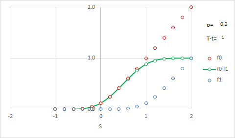
Variation of f0, f1 and (f0-f1) with σ
σ changes the shape of the framework. If I reduce σ from 0.9 to 0.3, f0 and f1 move down and all three curves are closer to their values at expiration. That is the expected behavior for these three option positions.
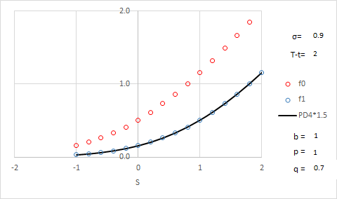
Variation of f0, f1 and (f0-f1) with T-t:
Time to expiration (T-t) also changes the shape of the frame. Initially, I set it to 1 to help expose the f’s. If it is now increased from 1 year to 2 years with σ=0.9, f0 and f1 move up, their curvatures broaden, and the tug factor (green) broadens. These are again the expected behaviors for these three option positions.
Calculating RIN price
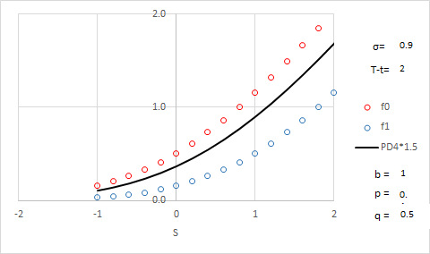
The above discussion all involved the framework. To actually calculate the RIN price, we must now assess the probability the blender’s tax credit will remain in effect. p=1.0 means 100% probability the tax credit will stay in effect. With p=1.0 and r=0, the “wet” D4 RIN price is the black curve below, equal to the blue curve:
If we instead set p=0.4, the RIN price is tugged up toward the red curve by the amount of the tug term reflecting a chance the tax credit will go away in the future.
With this insight on model structure, the movement of RIN prices can be better understood, studied and predicted.
Conclusions
- By considering a special case, the IMS model equation can be seen to consist of two option price curves and a “tug term” that pulls the RIN price between them.
- The two option price curves capture uncertainty on the future prices of diesel and biodiesel.
- The tug term depends on all the variables that affect the two option price curves and on the probability of future change in the blender’s tax credit.
- This insight helps understand and predict the factors that change RIN prices.
Recommendation
Considering the importance of RIN prices for profitability, every company affected by RINs should have at least one person with good understanding of RINs pricing including how to use the IMS RINs price model which is based on economic fundamentals and has been proven to accurately model real-world RIN prices. The first step in getting this capability is to get Hoekstra Research Report 10.
Recommendation
Anyone with a stake in RINs pricing and economics should get Hoekstra Research Report 10 which includes the Hoekstra ATTRACTOR spreadsheet spreadsheet that accurately calculates D4T, the theoretical RIN price, tracks it versus quoted market prices, and predicts how RIN prices will change with the variables that affect them. Why not send a purchase order today?
George Hoekstra george.hoekstra@hoekstratrading.com +1 630 330-8159
Anyone with a stake in RINs pricing and economics should get Hoekstra Research Report 10
[1] NOTE to Jim Stock: The tug term (f0 – f1 )p, multiplied by e^(-r) /1.5 is the “interesting gap” we were discussing when we saw the spreadsheet model RIN prices shift up and to the left when I decreased p from 1 to 0 with b=1. That gap depends on p, s, and all the parameters that affect the f’s.
george.hoekstra@hoekstratrading.com +1 630 330-8159